File	Description
Application.h	A C++ source code file containing a class declaration.
Application.cpp	A C++ source code file containing a class definition/implementation.
Makefile	A file containing instructions on how to build the application.
main.cpp	The application source code where the main function is defined.
Pi3 Image Processing.spa_binary_graph	A simplified binary version of the document you made in the Shader application. There is only one of these for each document you export.
Program-E7274A5C-F421-4C62-9E3F-8E9F58E3E419.spa_binary_node	A simplified binary version of the <Program> node in the document. Other files ending in .spa_binary_node represent other document nodes.

// #version 120
// The version number is automatically injected by the application.
// It is included above for reference purposes only.
#include <SPA_Version.glsl>

varying vec4 fs_position;
varying vec2 fs_texcoord;
varying vec3 fs_normal;
varying vec4 fs_color;
varying vec3 fs_normalViewspace;
varying vec3 fs_positionViewspace;

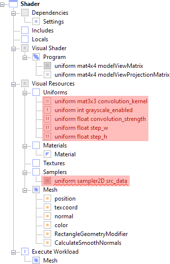
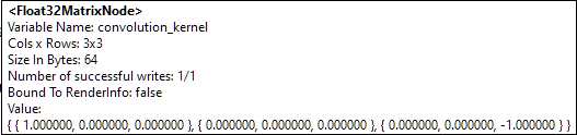
uniform mat3 convolution_kernel;
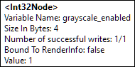
uniform int grayscale_enabled;
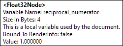
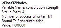
uniform float convolution_strength;
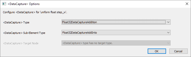
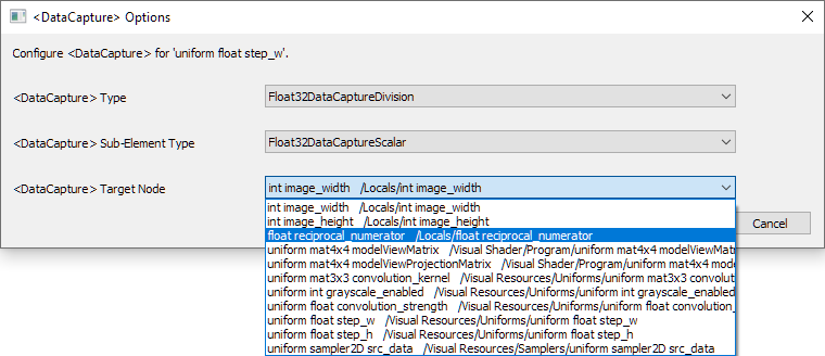
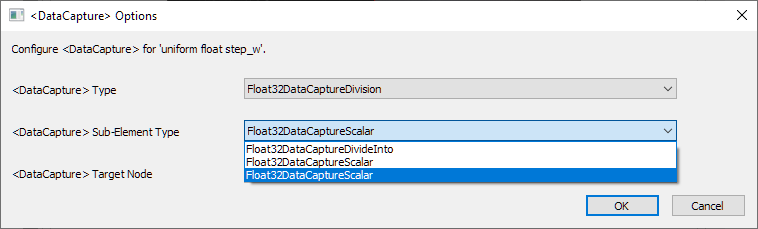
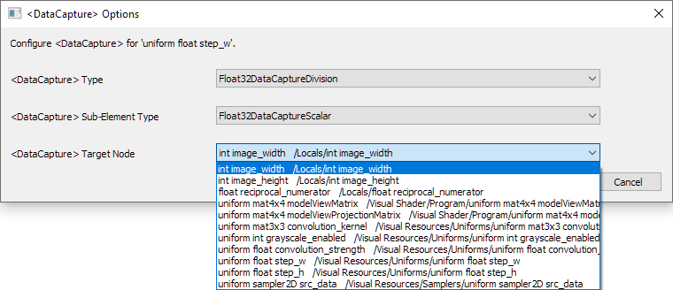
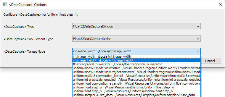
uniform float step_w;
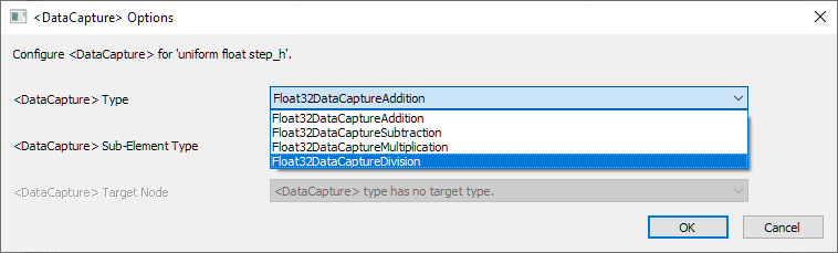
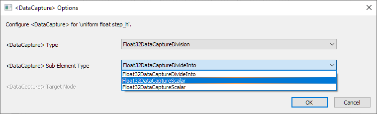
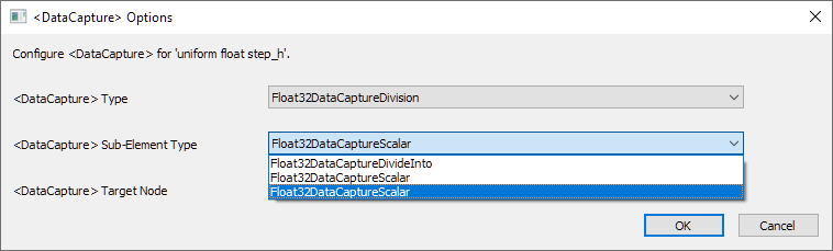
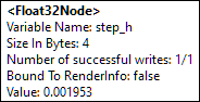
uniform float step_h;

const int KERNEL_SIZE = int( 9 );
float kernel[KERNEL_SIZE];
vec2 offset[KERNEL_SIZE];

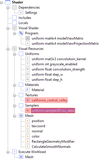
uniform sampler2D src_data;

void main(void)
{
   vec4 convolution;
   vec4 temp;
   float sum = 1.0;

   offset[0] = vec2( -step_w, -step_h );    offset[3] = vec2( -step_w, 0.0 );     offset[6] = vec2( -step_w, step_h );
   offset[1] = vec2( 0.0, -step_h );        offset[4] = vec2( 0.0, 0.0 );         offset[7] = vec2( 0.0, step_h );
   offset[2] = vec2( step_w, -step_h );     offset[5] = vec2( step_w, 0.0 );      offset[8] = vec2( step_w, step_h );

   kernel[0] = convolution_kernel[0][0] * convolution_strength;
   kernel[1] = convolution_kernel[0][1] * convolution_strength;
   kernel[2] = convolution_kernel[0][2] * convolution_strength;
   kernel[3] = convolution_kernel[1][0] * convolution_strength;
   kernel[4] = convolution_kernel[1][1] * convolution_strength;
   kernel[5] = convolution_kernel[1][2] * convolution_strength;
   kernel[6] = convolution_kernel[2][0] * convolution_strength;
   kernel[7] = convolution_kernel[2][1] * convolution_strength;
   kernel[8] = convolution_kernel[2][2] * convolution_strength;

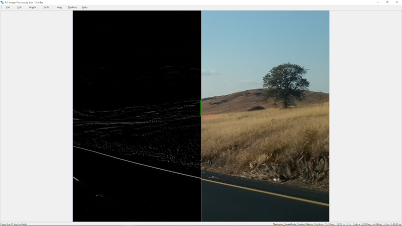
   if( fs_texcoord.s < 0.5 )
   {
      for( int i = 0; i < KERNEL_SIZE; i++ )
      {
         temp = texture2D( src_data, fs_texcoord.st + offset[i] );

         // If the grayscale flag is enabled, calculate the filter
         // based on the intensity of the pixels rather than the color value.
         // Otherwise process the rgb channels.
         if( grayscale_enabled > 0 )
         {
            float intensity = ( ( 0.299 * temp.r ) + ( 0.587 * temp.g ) + ( 0.114 * temp.b ) );
            convolution += vec4( intensity ) * kernel[i];
         }
         else
         {
            convolution += temp * kernel[i];
         }

         sum += kernel[i];
      }

      sum = max( sum, 1.0 );
      convolution = clamp( convolution / sum, vec4( 0.0 ), vec4( 1.0 ) );
   }
   else
   if( fs_texcoord.s > 0.502 )
   {
      convolution = texture2D( src_data, fs_texcoord.xy );
   }
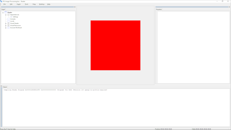
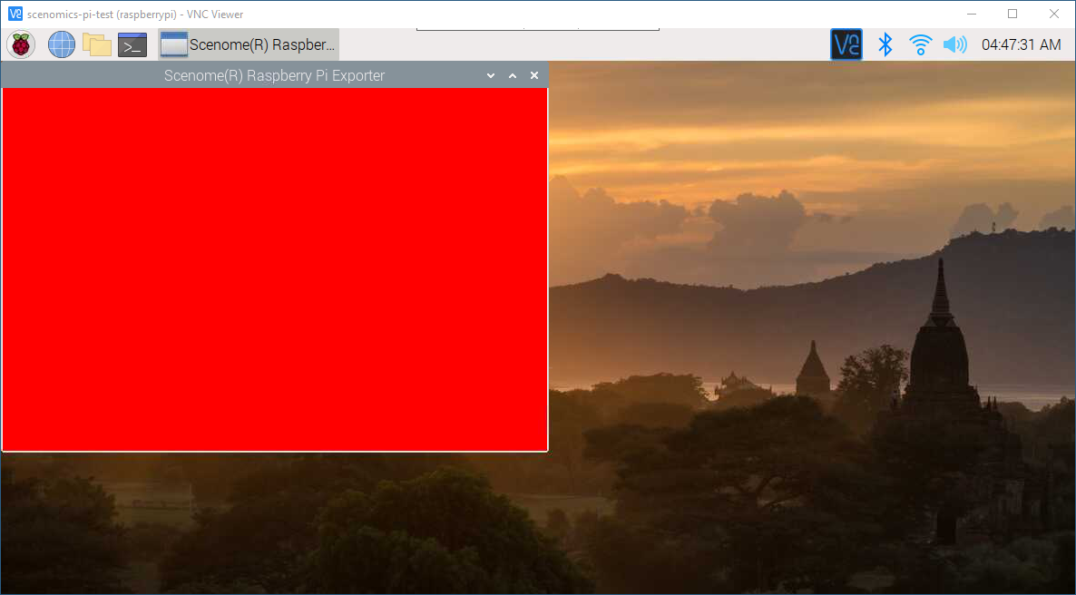
   else
   {
      convolution = vec4( 1.0, 0.0, 0.0, 1.0 );
   }

   gl_FragColor = convolution;
}

Create Image Processing Shader For Raspberry Pi 3B+

Start The Shader Application

Create A New Document

Test Export Functionality

Examine The New Document

Examine The <Program>

Copy Fragment Shader Path

Modify Fragment Shader

Rebuild The Document

Examine The Document

Load Texture From Disk

Create 'image_width' Declaration

Add <DataCapture>: int image_width

Create 'image_height' Declaration

Add <DataCapture>: int image_height

Create 'reciprocal_numerator' Declaration

Set Uniform: uniform mat3x3 convolution_kernel

Set Uniform: uniform int grayscale_enabled

Set Uniform: uniform float convolution_strength

Add <DataCapture>: uniform float step_w

Add <DataCapture>: uniform float step_h

View Results

Export To Raspberry® Pi 3B+